If you read the post about Boolean algebra, you might have noticed a substantial limitation: it can only deal with binary (True/False) variables.
How, then, can you make predictions for quantitative variables? You probably already know the answer.
If you are going to the seaside by car, the seaside is 100 km away, and you are driving at 50 km/h, how long will it take you to reach the seaside?
 Photo by Zach Dischner
2 hours, of course.
To introduce a new tool - differential equations - here is another way to see the problem.
Let $x$ be your position on the way to the seaside. $x=0$ is the starting point, $x=100$ is the arrival.
Your speed is the rate of change of $x$, denoted as $\frac{dx}{dt}$.
$$ \frac{dx}{dt}=50$$
This is a differential equation. It describes the rate of change of a variable. This example is simple, because the differential equation is constant, but it could potentially be more complex and depend on your current position, e.g.:
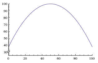
$$ \frac{dx}{dt}=100-\frac{1}{40}(x-50)^2$$

Even if the differential equation is complex, you can still use it to plot the state of the system (e.g.: your position) at any instant in the future. This is what makes differential equations powerful.
This is a process called “numerical integration”, and is generally handled by dedicated computer programs, but the idea is quite simple:
- Check your current position in the simulation.
- Compute your current speed.
- Compute how far you are going to travel at that speed in one second.
- Add the result of step 3 to the value observed at step 1.
- Update your current position in the simulation based on the result of step 4.
- Go to step 1 and repeat. You then just have to look at when $x$ becomes greater than 100 to know when you will arrive.
 Photo by NeilsPhotography
Banner photo by Internet Archive Book Images
